
Turing machine


A Turing machine is a device that manipulates symbols on a strip of tape according to a table of rules. Despite its simplicity, a Turing machine can be adapted to simulate the logic of any computer algorithm and is particularly useful in explaining the functions of a CPU within a computer.
Originally it was defined by the English mathematician Alan Turing as an «automatic machine» in 1936 in the journal Proceedings of the London Mathematical Society. The Turing machine is not designed as a practical computing technology, but as a hypothetical device that represents a computing machine. Turing machines help scientists understand the limits of mechanical computation.
Turing gave a succinct definition of experiment in his 1948 essay, "Intelligent Machines." Referring to his 1936 publication, Turing wrote that the Turing machine, here called a computing logic machine, consisted of:
... an unlimited memory capacity obtained in the form of an infinite tape marked with squares, in each of which a symbol could be printed. At any time there is a symbol on the machine; called the symbol read. The machine can alter the read symbol and its behavior is partly determined by that symbol, but symbols in other places of the tape do not affect the behavior of the machine. However, the tape can be moved forward and backward through the machine, being one of the elementary operations of the machine. Therefore any symbol on the tape can finally have a chance.Turing (1948, p. 61.)
A Turing machine that is capable of simulating any other Turing machine is called a Universal Turing Machine (UTM, or simply a Universal Machine). A more mathematically oriented definition, with a similar "universal" nature, was advanced by Alonzo Church, whose work on lambda calculus intertwines with Turing's in a formal theory of computation known as Church's thesis. -Turing. The thesis points out that Turing machines do, in fact, capture the informal notion of an effective method in logic and mathematics and provide a precise definition of an algorithm or 'mechanical procedure'.
The importance of the Turing machine in the history of computing is twofold: first, the Turing machine was one of the first (if not the first) theoretical models for computers, seeing the light of day in 1936. Second, By studying its abstract properties, the Turing machine has served as the basis for much theoretical development in computer science and complexity theory. One reason for this is that Turing machines are simple, and therefore amenable to analysis. That said, it should be noted that Turing machines are not a practical model for computing on real machines, which require faster models such as those based on RAM.
History


Alan Turing introduced the concept of the Turing machine in the work On computable numbers, with an application to the Entscheidungsproblem, published by the London Mathematical Society in 1936, in which the question was studied. raised by David Hilbert about whether mathematics is decidable, that is, if there is a defined method that can be applied to any mathematical sentence and that tells us if that sentence is true or not. Turing devised a formal model of a computer, the Turing machine, and showed that there were problems that a machine could not solve.
With this extremely simple device it is possible to perform any computation that a digital computer is capable of performing.)
By means of this theoretical model and the analysis of the complexity of the algorithms, it was possible to categorize computational problems according to their behavior, thus appearing, the set of problems called P and NP, whose solutions can be found in polynomial time by deterministic and non-deterministic Turing machines, respectively.
Precisely, the Church-Turing thesis formulated by Alan Turing and Alonzo Church, independently in the mid-20th century, characterizes the informal notion of computability with computing using a Turing machine.
The underlying idea is the concept that a Turing machine can be seen as an automaton executing a formally defined effective procedure, where the working memory space is unlimited, but at any given time only a finite part is accessible.
Informal description


The Turing machine mathematically models a machine that operates mechanically on a tape. On this tape are symbols that the machine can read and write, one at a time, using a tape read/write head. The operation is completely determined by a finite set of elementary instructions like "in state 42, if the symbol seen is 0, write a 1; If the symbol seen is 1, it changes to state 17; in state 17, if the symbol seen is 0, it writes a 1 and changes to state 6; etc". In the original article ("On Computable Numbers with an Application to the Entscheidungsproblem"), Turing imagines not a mechanism, but a person he calls the "computer", who slavishly executes these deterministic mechanical rules (or as Turing puts it, "in a half-hearted way").
More precisely, a Turing machine consists of:
- One tape that is divided into cells, one next to the other. Each cell contains a symbol of some finite alphabet. The alphabet contains a special symbol called white (here written as 'B') and one or more additional symbols. The tape is supposed to be arbitrarily extendable to the left and to the right, that is, the Turing machine is always provided with as much tape as you need for your computer. Cells that have not been previously written are assumed to be filled with the white symbol. In some models the tape has a left end marked with a special symbol; the tape extends or is indefinitely extendable to the right.
- A head you can read and write symbols on the tape and move the tape to the left and right one (and only one) cell at a time. In some models the head moves and the tape is stationary.
- A status record which stores the state of the Turing machine, one of the finite states. There is a special initial state with which the status record is started. Turing writes that these states replace the "state of mind" in which he would normally be a person performing calculations.
- One Table finite instructions (called occasionally as Action table or transition function). The instructions are usually 5-tuples: qiaj→qi1aj1dk(sometimes 4-tuplas), which, given the state (q)i) in which the machine is currently and the symbol (laughs)j) that is being read on the tape (the symbol currently below the head) tells the machine to do the following in sequence (for 5-tuplate models):
- Delete or write a symbol (replace toj with aj1), And then
- Move the head (which is described by dk and may have the values: 'L' for a step to the left, or 'R' for a step to the right, or 'N' to stay in the same place) and then
- Assume the same or a new state as prescribed (see the state qi1).
- In 4-tupla models, they are specified as separate instructions: delete or write a symbol (toj1) and move the head to the left or right (dk). Specifically, the table indicates to the machine: (ia) delete or write a symbol or (ib) move the head to the left or right, and then (ii) assume the same or a new state, but not the two actions (ia) and (ib) in the same instruction. In some models, if there is no entry in the table for the current combination of symbol and status, the machine will stop; other models require that all entries be filled.
Note that each part of the machine — its state and collections of symbols — and its actions — print, erase, tape motion — is finite, discrete, and distinguishable; it's the potentially unlimited amount of tape that gives you an unlimited amount of storage space.
Formal definition
A Turing machine is a computational model that automatically performs a read/write on an input called a tape, generating an output on it.
This model consists of an entry alphabet and one output, a special symbol called white (normally b, Δ Δ {displaystyle Delta } or 0), a set of finite states and a set of transitions between those states. Its operation is based on a transition function, which receives a Initial status and a string of characters (the tape, which can be infinite) belonging to the input alphabet. The machine is reading a tape cell in each step, erasing the symbol in which its head is positioned and writing a new symbol belonging to the output alphabet, then scrolling the head to the left or right (only one cell at a time). This is repeated as indicated in the transition function, to finally stop in a Final status or acceptance, thus representing the exit.

A Turing machine with a single tape can be defined as a 7-tuple
- M=(Q,・ ・ ,Interpreter Interpreter ,s,b,F,δ δ ),{displaystyle M=(Q,SigmaGammas,b,F,delta),!}

where:
- Q{displaystyle Q!} It's a finite set of states.
- ・ ・ {displaystyle sigma !} is a finite set of symbols other than the blank space, called machine or input alphabet.
- Interpreter Interpreter {displaystyle Gamma !} is a finite set of tape symbols, called tape alphabet (・ ・ Interpreter Interpreter {displaystyle Sigma subseteq Gamma }).
- s한 한 Q{displaystyle sin Q} It's the initial state.
- b한 한 Interpreter Interpreter {displaystyle bin Gamma } is a symbol called white, and it is the only symbol that can be repeated an infinite number of times.
- F Q{displaystyle Fsubseq Q} is the set of final acceptance states.
- δ δ :Q× × Interpreter Interpreter → → Q× × Interpreter Interpreter × × {L,R!{displaystyle delta:Qtimes Gamma rightarrow Qtimes Gamma times {L,R}} is a partial function called the transition function, where L{displaystyle L!} It's a movement to the left and R{displaystyle R!} It's the right move.


There are many alternative definitions in the literature, but they all have the same computer power, for example the symbol can be added. S{displaystyle S!} as a symbol of "no movement" in a computing step.

How the Turing Machine Works
The Turing machine consists of a read/write head and an infinite tape where the head reads the content, erases the old content, and writes a new value. The operations that can be performed on this machine are limited to:
- Move the reader/write head to the right.
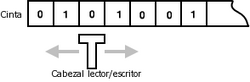 Visualization of a Turing machine, in which you see the head and the tape that you read.
 - Move the reader/write head to the left.

The computation is determined from a state table of the form:
- (state, value) → → {displaystyle rightarrow } (new state, new value, direction)

This table takes as parameters the current state of the machine and the character read from the tape, giving the direction to move the spindle, the new state of the machine and the value to write on the tape.
Memory is the machine's tape that is divided into workspaces called cells, where symbols can be written and read. Initially all cells contain a special symbol called "blank". The instructions that determine the operation of the machine have the form, "if we are in the state x reading the position y, where the symbol is written z, then this symbol should be replaced by this other symbol, and read the next cell, either to the left or to the right".
The Turing machine can be considered as an automaton capable of recognizing formal languages. In this sense, it is capable of recognizing recursively enumerable languages, according to Chomsky's hierarchy. Its power is, therefore, superior to other types of automata, such as the finite automaton, or the automaton with a battery, or equal to other models with the same computational power.
Representation as state diagram
Turing machines can be represented by particular graphs, also called finite state diagrams, as follows:


Interpreter Interpreter ={X,And,Z,B!{displaystyle Gamma ={X,Y,Z,B}} being B{displaystyle B} the symbol called "white." This machine recognizes the regular expression of form anbncn{displaystyle a^{n}b^{n}c^{n} with =0}" xmlns="http://www.w3.org/1998/Math/MathML">n▪0{displaystyle n vocabulary=0}


- The states are represented as vertices, labeled with their name inside.
- A transition from one state to another, is represented by a directed edge that binds these vertices, and is labeled by symbol that reads the head/symbol that will write the head, movement of the head.
- The initial state is characterized by having an edge that comes to it and does not come from any other vertex.
- He or the final states are represented by vertices that are locked in turn by another circumference.
Instant Overview
It's a sequence of form α α 1qα α 2{displaystyle alpha _{1}qalpha _{2}!} where α α 1,α α 2한 한 Interpreter Interpreter ↓ ↓ {displaystyle alpha _{1},alpha _{2}in Gamma ^{*}} and q한 한 Q{displaystyle qin Q} that writes the status of a Turing machine. The tape contains the string α α 1α α 2{displaystyle alpha _{1}alpha _{2}!} followed by infinite whites. The head signals the first symbol α α 2{displaystyle alpha _{2}}.


For example, for the Turing machine
- MT=({p,q!,{0,1!,{0,1,x!,p,Δ Δ ,{q!,δ δ ),{displaystyle MT=({p,q},{0,1},{0,1,x},p,Delta{q},delta),!}

with transitions
- δ δ (p,1)=(p,x,R),δ δ (p,0)=(p,0,R)andδ δ (p,Δ Δ )=(q,Δ Δ ,R).{displaystyle {begin{aligned}delta (p,1) stranger=(p,x,R),\delta (p,0) nightmare=(p,0,R){text{ y}}delta (p,Delta) fake=(q,DeltaR).end{aligned}}

The snapshot description for tape 1011 is:
- p1011Δ Δ Δ Δ ...... {displaystyle p1011Delta ldots }
- xp011Δ Δ Δ Δ ...... {displaystyle xp011Delta ldots }
- x0p11Δ Δ Δ Δ ...... {displaystyle x0p11Delta ldots }
- x0xp1Δ Δ Δ Δ ...... {displaystyle x0xp1Delta ldots }
- x0xxpΔ Δ Δ Δ ...... {displaystyle x0xxpDelta ldots }
- x0xxqΔ Δ Δ Δ ...... {displaystyle x0xxqDelta ldots }


Example
We define a Turing machine on the alphabet {0,1!{displaystyle {0,1}}where 0 represents the white symbol. The machine will begin its process on a "1" symbol of a series. The Turing machine will copy the number of "1" symbols you find until the first target behind that white symbol. That is, position the head over the 1 located at the left end, turn the number of symbols 1, with a 0 in the middle. Thus, if we have the "111" entry will return "1110111", with "1111" will return "111101111", and so on.

The set of states is {s1,s2,s3,s4,s5!{displaystyle {s_{1},s_{2},s_{3},s_{4},s_{5}}}! and the initial state is s1{displaystyle s_{1}!}. The table that describes the transition function is the Next:


| State | Symbol read | Written symbol | Mov. | State sig. |
|---|---|---|---|---|
| s1{displaystyle s_{1},!} | 1 | 0 | R{displaystyle R,!} | s2{displaystyle s_{2},!} |
| s2{displaystyle s_{2},!} | 1 | 1 | R{displaystyle R,!} | s2{displaystyle s_{2},!} |
| s2{displaystyle s_{2},!} | 0 | 0 | R{displaystyle R,!} | s3{displaystyle s_{3},!} |
| s3{displaystyle s_{3},!} | 0 | 1 | L{displaystyle L,!} | s4{displaystyle s_{4},!} |
| s3{displaystyle s_{3},!} | 1 | 1 | R{displaystyle R,!} | s3{displaystyle s_{3},!} |
| s4{displaystyle s_{4},!} | 1 | 1 | L{displaystyle L,!} | s4{displaystyle s_{4},!} |
| s4{displaystyle s_{4},!} | 0 | 0 | L{displaystyle L,!} | s5{displaystyle s_{5},!} |
| s5{displaystyle s_{5},!} | 1 | 1 | L{displaystyle L,!} | s5{displaystyle s_{5},!} |
| s5{displaystyle s_{5},!} | 0 | 1 | R{displaystyle R,!} | s1{displaystyle s_{1},!} |


The operation of a computation of this machine can be shown with the following example (in bold the position of the reading/writing head is highlighted):
| Step | State | Ribbon |
|---|---|---|
| 1 | s1{displaystyle s_{1},!} | 11 |
| 2 | s2{displaystyle s_{2},!} | 01 |
| 3 | s2{displaystyle s_{2},!} | 010 |
| 4 | s3{displaystyle s_{3},!} | 0100 |
| 5 | s4{displaystyle s_{4},!} | 0101 |
| 6 | s5{displaystyle s_{5},!} | 0101 |
| 7 | s5{displaystyle s_{5},!} | 0101 |
| 8 | s1{displaystyle s_{1},!} | 1101 |
| 9 | s2{displaystyle s_{2},!} | 1001 |
| 10 | s3{displaystyle s_{3},!} | 1001 |
| 11 | s3{displaystyle s_{3},!} | 10010 |
| 12 | s4{displaystyle s_{4},!} | 10011 |
| 13 | s4{displaystyle s_{4},!} | 10011 |
| 14 | s5{displaystyle s_{5},!} | 10011 |
| 15 | s1{displaystyle s_{1},!} | 11011 |
| Stop. | ||
The machine performs its process through a loop, in the initial state s1{displaystyle s_{1}!}replace the first one with a 0, and move to the state s2{displaystyle s_{2}!}, with which it advances to the right, jumping symbols 1 to 0 (which must exist), when it finds it passes to the state s3{displaystyle s_{3}!}, with this state progresses jumping the 1st to find another 0 (the first time there will be no 1). Once on the right end, add a 1. Then begins the return process; with s4{displaystyle s_{4}!} back to the left jumping the 1, when you find a 0 (in the middle of the sequence) s5{displaystyle s_{5}!} that continues to the left jumping the 1 to the 0 that was written at the beginning. It is replaced again this 0 by 1, and passes to the next symbol, if it is a 1, it is passed to another iteration of the loop, passing to the s1 state again. If it is a 0 symbol, it will be the central symbol, so the machine stops when the compute is finished.


Equivalent modifications
One reason to accept the Turing machine as a general model of computing is that the model we have defined above is equivalent to many modified versions that at first appear to increase computational power.
Turing machine with waiting motion
The transition function of the simple TM is defined by
- δ δ :Q× × Interpreter Interpreter → → Q× × Interpreter Interpreter × × {L,R!,{displaystyle delta:Qtimes Gamma rightarrow Qtimes Gamma times {L,R},}

which can be modified as
- δ δ :Q× × Interpreter Interpreter → → Q× × Interpreter Interpreter × × {L,R,S!.{displaystyle delta:Qtimes Gamma rightarrow Qtimes Gamma times {L,R,S}. !

Where S{displaystyle S!} means "to remain" or "wait", that is not to move the head of reading/writing. So, δ δ (q,σ σ )=(p,σ σ ♫,S){displaystyle delta (q,sigma)=(p,sigma',S)!} means that it passes from the state q Al p, it is written σ σ ♫{displaystyle sigma} in the current cell and the head stays on the current cell.


Turing machine with infinite tape on both sides
This modification is denoted as a simple MT, which makes it different is that the tape is infinite both on the right and on the left, which allows to make initial transitions as well as δ δ (q0,x)=(q1,and,L){displaystyle delta (q_{0},x)=(q_{1},y,L)!}.

Turing machine with multitrack tape
It is one that by means of which each cell of the tape of a simple machine is divided into subcells. Each cell is thus capable of containing several ribbon symbols. For example, the ribbon in the figure has each cell subdivided into three subcells.
This tape is said to have multiple tracks since each cell of this Turing machine contains multiple characters, the contents of the cells of the tape can be represented by ordered n-tuples. The movements that this machine makes will depend on its current state and on the n-tuple that represents the contents of the current cell. It is worth mentioning that it has a single head just like a simple TM.
Multi-tape Turing machine
A TM with more than one tape consists of a finite controller with k read/write heads and k tapes. Each tape is infinite in both directions. The TM defines its movement depending on the symbol that each of its heads is reading, it gives substitution rules for each of the symbols and direction of movement for each of the heads. Initially the TM starts with the input on the first tape and the rest of the tapes are blank.
Multidimensional Turing Machine
A multidimensional TM is one whose tape can be seen as extending infinitely in more than one direction, the most basic example would be a two-dimensional machine whose tape would extend infinitely up, down, right, and left.
In the two-dimensional modification of TM shown in the figure, two new head movements {U,D} (ie up and down) are also added. In this way, the definition of the movements carried out by the spindle will be {L,R,U,D}.
|


Deterministic and non-deterministic Turing machine
The input of a Turing machine is determined by the current state and the symbol read, a pair (state, symbol), being the change of state, the writing of a new symbol and the movement of the head, the actions to take based on an input. In the case that for each possible pair (state, symbol) there is at most one possibility of execution, it will be said that it is a deterministic Turing machine, while in the case that there is at least one pair (state, symbol) with more than one possible combination of actions it will be said that it is a non-deterministic Turing machine.
The transition function δ δ {displaystyle delta } in the non-determinist case, it is defined as follows:

- δ δ :Q× × Interpreter Interpreter → → P(Q× × Interpreter Interpreter × × {L,R!){displaystyle delta:Qtimes Gamma rightarrow {mathcal {P}(Qtimes Gamma times {L,R})}

How does a non-deterministic machine know which action to take among several possible ones? There are two ways to look at it: one is to say that the machine is "the best guesser possible," that is, it always chooses the transition that will ultimately bring it to a final state of acceptance. The other is to imagine that the machine is 'cloned', branching into several copies, each of which follows one of the possible transitions. Whereas a deterministic machine follows a single "computational path", a non-deterministic machine has a "computational tree". If any of the branches of the tree end in an accepting state, the machine is said to accept the input.
The computing capacity of both versions is equivalent; it can be demonstrated that given a non-determinist Turing machine there is another equivalent deterministic Turing machine, in the sense that it recognizes the same language, and vice versa. However, the speed of execution of both formalisms is not the same, since if a non-determinist machine M recognizes a certain word of size n in a while O(t(n)){displaystyle O(t(n)}the equivalent determinist machine will recognize the word in a time O(2t(n)){displaystyle O(2^{t(n)})!}. In other words, non-determinism will reduce the complexity of solving problems, allowing to solve, for example, problems of exponential complexity in a polynomic time.


Halting problem
The halting problem or halting problem for Turing machines consists of: given a MT M and a word w, determine whether M will terminate in a finite number of steps when executed using w as entrance.
Alan Turing, in his famous paper «On computable numbers, with an application to the Entscheidungsproblem» (1936), showed that the Turing machine stall problem is undecidable, in the sense that no Turing machine can solve it.
Coding a Turing machine
Every Turing machine can be encoded as a finite binary sequence, i.e. a finite sequence of zeros and one. To simplify encoding, we assume that all MT has a single initial state denoted by q1{displaystyle q_{1}!}and a single final state scored q2{displaystyle q_{2}!}. We'll have to get an MT. M form


- Interpreter Interpreter ={s1,s2,...... ,sm,...... ,sp!{displaystyle Gamma ={s_{1},s_{2},ldotss_{m},ldotss_{p}{p}}!} where s1{displaystyle s_{1}} represents the white symbol 0, Δ Δ {displaystyle Delta } or b (as you wish to denote),
- ・ ・ ={s2,...... ,sm!{displaystyle sigma ={s_{2},ldotss_{m}}!} it's entry alphabet and
- {sm+1,...... ,sp!{displaystyle {s_{m+1},ldotss_{p}}!} are the auxiliary symbols used by M (each MT uses its own finite collection of auxiliary symbols).


All of these symbols are encoded as sequences of ones:
| Symbol | Codification |
|---|---|
| s1{displaystyle s_{1}} | 1 |
| s2{displaystyle s_{2}} | 11 |
| s3{displaystyle s_{3}} | 111 |
| . . . | . . . |
| sm{displaystyle s_{m}} | 1m{displaystyle 1^{m}} |
| sp{displaystyle s_{p}} | 1p{displaystyle 1^{p}} |


The states of an MT q1,q2,q3,...... ,qn{displaystyle q_{1},q_{2},q_{3},ldotsq_{n}}! are also encoded with sequences of some:

| Symbol | Codification |
|---|---|
| q1(inicial){displaystyle q_{1}({rm {initial}}}}}} | 1 |
| q2(final){displaystyle q_{2}({rm {final)}}} | 11 |
| . . . | . . . |
| qn{displaystyle q_{n}} | 1n{displaystyle 1^{n}} |


Displacement guidelines R{displaystyle R!}, L{displaystyle L!} and S{displaystyle S!} are encoded with 1, 11, 111, respectively. A transition δ δ (q,a)=(p,c,R){displaystyle delta (q,a)=(p,c,R)!} is coded using zeros as separators between states, the symbols of the tape alphabet and the scrolling guideline R{displaystyle R!}. Thus, the transition δ δ (q3,s2)=(q5,s3,R){displaystyle delta (q_{3},s_{2})=(q_{5},s_{3},R)!} encoded as


- 01110110111110111010.{displaystyle 01110110111110111010. !

In general, the codification of any transition δ δ (qi,sk)=(qj,sl,R){displaystyle delta (q_{i},s_{k})=(q_{j},s_{l},R)!} That's it.

- 01i01k01j01l01t,{displaystyle 01^{i}01^{k}{j}01^{l}01^{t},}

where t한 한 {1,2,3!{displaystyle tin {1,2,3}!}according to the address derecha(R),izquierda(L),esperar(S){displaystyle mathrm {right} (R), mathrm {left} (L), mathrm {wait} (S)}.


A MT is codified by consecutively writing the sequences of modifications of all its transitions. More precisely, the encoding of an MT M is shape C1C2...... Ci{displaystyle C_{1}C_{2}ldots C_{i}}, where Ci{displaystyle C_{i}!} is the encoding of the i{displaystyle i}-thousand transition M. Since the order in which the transitions of an MT are represented is not relevant, the same MT has several different encodings. This does not represent any practical or conceptual disadvantage since codifications are not intended to be unique.


Universal Turing Machine
A Turing machine computes a certain partial function of definite and unambiguous character, defined on the sequences of possible strings of symbols of its alphabet. In this sense it can be considered as equivalent to a computer program, or an algorithm. However, it is possible to encode the table that represents a Turing machine, in turn, as a sequence of symbols in a given alphabet; therefore, we can build a Turing machine that accepts as input the table representing another Turing machine, and thus simulates its behavior.
In 1947, Turing stated:
It can be shown that it is possible to build a special machine of this type that can perform the work of all others. This special machine can be called a universal machine.
This encoding of tables as strings opens up the possibility of Turing machines behaving like other Turing machines. However, many of its possibilities are undecidable, since they do not admit an algorithmic solution. For example, an interesting problem is to determine if any Turing machine will stop in a finite time on a given input; known as the stopping problem, which Turing showed to be undecidable. In general, any non-trivial question about the behavior or output of a Turing machine can be shown to be an undecidable problem.
The concept of a universal Turing Machine is related to that of a basic operating system, since it can execute any computable instruction on it.
Quantum Turing Machine

In 1985, Deutsch presented the design of the first Quantum Machine based on a Turing machine. To this end, he enunciated a new variant of the Church-Turing thesis, giving rise to the so-called "Church-Turing-Deutsch principle".
The structure of a quantum Turing machine is very similar to that of a classical Turing machine. It is composed of the three classic elements:
- An infinite memory tape where each element is a qubit.
- A finite processor.
- A head.
The processor contains the set of instructions that is applied to the element of the tape pointed to by the head. The result will depend on the qubit of the tape and the state of the processor. The processor executes one instruction per unit of time.
The memory tape is similar to that of a traditional Turing machine. The only difference is that each element on the quantum machine's ribbon is a qubit. The alphabet of this new machine is formed by the space of values of the qubit. The head position is represented by an integer variable.
Equivalent models
Two mathematical models equivalent to those of Turing machines are Post machines, created in parallel by Emil Leon Post, and the lambda calculus, introduced by Alonzo Church and Stephen Kleene in the 1930s, and also used by Church to demonstrate in 1936 the Entscheidungsproblem.
Contenido relacionado
Annex: Home computers by category
Windows 2000
Twin prime number