Pareto distribution

ImprimirCitar

In probability theory and statistics, the Pareto distribution is a continuous probability distribution with two parameters, which has applications in disciplines such as sociology, geophysics and economics. It was formulated by the civil engineer, economist and sociologist Vilfredo Pareto, although in certain areas of study reference is made to Bradford's law. It should be noted that the discrete equivalent of the Pareto distribution is the zeta distribution (Zipf's law).

When the distribution of Pareto is used in a model on the distribution of wealth, the parameter ${displaystyle alpha }$ is known as the Pair Index.

Definition

Notation

Yeah. $X$ is a continuous random variable with distribution Couple with parameters $0}" xmlns="http://www.w3.org/1998/Math/MathML">α α ▪0{displaystyle alpha 한0}0}" aria-hidden="true" class="mwe-math-fallback-image-inline" src="https://wikimedia.org/api/rest_v1/media/math/render/svg/edd4f784b6e8bb68fa774213ceacbab2d97825dc" style="vertical-align: -0.338ex; width:5.749ex; height:2.176ex;"/>$ and $0}" xmlns="http://www.w3.org/1998/Math/MathML">xm▪0{displaystyle x_{m} 20050}0}" aria-hidden="true" class="mwe-math-fallback-image-inline" src="https://wikimedia.org/api/rest_v1/media/math/render/svg/918b5f040802b51d44b4d982f25a250f8ecf0db3" style="vertical-align: -0.671ex; width:7.266ex; height:2.509ex;"/>$ Then we write ${displaystyle Xsim operatorname {Pareto} (alphax_{m})}$ .

Density function

The density function of a random variable ${displaystyle Xsim operatorname {Pareto} (alphax_{m})}$ That's it.

{displaystyle f_{X}(x)={frac {alpha x_{m}^{alpha }}{x^{alpha +1}}}}

for ${displaystyle x_{m}leq x}$ .

Cumulative Probability

The distribution function of a random variable ${displaystyle Xsim operatorname {Pareto} (alphax_{m})}$ It's, uh, stop. ${displaystyle x_{m}leq x}$ ,

{displaystyle F_{X}(x)=1-left({frac {x_{m}}{x}}right)^{alpha }}

Properties

Yeah. ${displaystyle Xsim operatorname {Pareto} (alphax_{m})}$ then the random variable $X$ satisfies some properties.

Media

The mean of the random variable $X$ That's it.

{displaystyle operatorname {E} [X]={frac {alpha x_{mathrm {m} }}{alpha -1}},}

with $1}" xmlns="http://www.w3.org/1998/Math/MathML">α α ▪1{displaystyle alpha 한1}1}" aria-hidden="true" class="mwe-math-fallback-image-inline" src="https://wikimedia.org/api/rest_v1/media/math/render/svg/17d81dbbc4786493c7b8548cc324a978d7cf5dbd" style="vertical-align: -0.338ex; width:5.749ex; height:2.176ex;"/>$ .

Variance

Variance of the random variable $X$

{displaystyle mathrm {Var} (X)={frac {alpha x_{m}^{2}}{(alpha -1)^{2}(alpha -2)}}}

for $2}" xmlns="http://www.w3.org/1998/Math/MathML">α α ▪2{displaystyle alpha 한2}2}" aria-hidden="true" class="mwe-math-fallback-image-inline" src="https://wikimedia.org/api/rest_v1/media/math/render/svg/432334d220d6e1b0340cc2a37531d0327494a8e2" style="vertical-align: -0.338ex; width:5.749ex; height:2.176ex;"/>$ .

Moments

The $n$ - that moment is only defined for $<math alttext="{displaystyle nn.α α {displaystyle n Âalpha } <img alt="{displaystyle n$ and in such a case it is

{displaystyle operatorname {E} [X^{n}]={frac {alpha x_{mathrm {m} }^{n}}{alpha -n}}}

Moment generating function

The moment generating function is

{displaystyle M_{X}(t)=alpha (-x_{mathrm {m} }t)^{alpha }Gamma (-alpha-x_{mathrm {m} }t)}

and is defined for values $<math alttext="{displaystyle tt.0{displaystyle t vis0} <img alt="{displaystyle t$ .

Degenerate case

The Dirac delta function is a limiting case of the Pareto density:

{displaystyle lim _{alpha rightarrow infty }f(x;alphax_{mathrm {m} })=delta (x-x_{mathrm {m} }).,}

Symmetric distribution

A Symmetrical Pareto Distribution can be defined according to:

x_{mathrm {m} }\0&{text{resto}}.end{cases}}}" xmlns="http://www.w3.org/1998/Math/MathML">f(x;α α ,xm)={(α α xmα α /2)日本語x日本語− − α α − − 1Yeah.日本語x日本語▪xm0other.{displaystyle f(x;alphax_{mathrm {m} })={begin{cases}(alpha x_{mathrm {m} }{alpha }{alpha }{alphah}{alphah}{alphah}{mathrm {m}{end}{.}{alphah.}{alphah.}{alphah.}{alphah.x_{mathrm {m} }\0&{text{resto}}.end{cases}}}" aria-hidden="true" class="mwe-math-fallback-image-inline" src="https://wikimedia.org/api/rest_v1/media/math/render/svg/e69cfa2899c69a7180290805bac398120369c782" style="vertical-align: -2.505ex; width:45.455ex; height:6.176ex;"/>

Generalized Pareto Distribution

The family of Generalized distributions of Couple (GPD) have three parameters ${displaystyle musigma ,}$ and ${displaystyle xi ,}$ .

The cumulative probability function is

{displaystyle F_{(ximusigma)}(x)={begin{cases}1-left(1+{frac {xi (x-mu)}{sigma }}right)^{-1/xi }&{text{si }}xi neq 0,\1-exp left(-{frac {x-mu }{sigma }}right)&{text{si }}xi =0.end{cases}}}

Stop. ${displaystyle xgeqslant mu }$ , with ${displaystyle xi geqslant 0,}$ and ${displaystyle xleqslant mu -sigma /xi }$ with $<math alttext="{displaystyle xi roga roga .0{displaystyle xi ₡0,} <img alt="{displaystyle xi$ Where ${displaystyle mu in mathbb {R} }$ is the parameter location, $0,}" xmlns="http://www.w3.org/1998/Math/MathML">σ σ ▪0{displaystyle sigma 한0,}0,}" aria-hidden="true" class="mwe-math-fallback-image-inline" src="https://wikimedia.org/api/rest_v1/media/math/render/svg/5a93bb4226a217819f9ef0467fbb3d47279a7910" style="vertical-align: -0.338ex; width:5.978ex; height:2.176ex;"/>$ is the parameter scale and ${displaystyle xi in mathbb {R} }$ is the parameter shape. Note that some references take the parameter shape Like ${displaystyle kappa =-xi ,}$ .

The probability density function is:

{displaystyle f_{(ximusigma)}(x)={frac {1}{sigma }}left(1+{frac {xi (x-mu)}{sigma }}right)^{left(-{frac {1}{xi }}-1right)}.}

{displaystyle f_{(ximusigma)}(x)={frac {sigma ^{frac {1}{xi }}}{left(sigma +xi (x-mu)right)^{{frac {1}{xi }}+1}}}.}

again, stop ${displaystyle xgeqslant mu }$ and ${displaystyle xleqslant mu -sigma /xi }$ Yeah. $<math alttext="{displaystyle xi roga roga .0{displaystyle xi ₡0,} <img alt="{displaystyle xi$

Occurrence and applications

General

Application of the accumulated probability distribution of Pareto to maximum daily rains.

Vilfredo Pareto originally used this distribution to describe the allocation of wealth among individuals, since it seemed to show quite well how more of the wealth in any society is owned by a smaller percentage of the people in that society. society. He also used it to describe the distribution of income. This idea is sometimes expressed more simply as the Pareto principle or the "80-20 rule", which says that 20% of the Population controls 80% of the wealth. However, the 80-20 rule corresponds to a particular value of α, and in fact, Pareto's data on British income taxes in his Cours d' économie politique indicate that approximately 30% of the population had about 70% of the income. The probability density function (PDF) at the beginning of this article shows that the "probability" The fraction of the population that owns a small amount of wealth per person is quite high, and then steadily declines as wealth increases. (However, the Pareto distribution is unrealistic for wealth at the lower end. In fact, net worth may even be negative.) This distribution is not limited to describing wealth or income, but many situations in which an equilibrium is found in the distribution of the "small" to "big". The following examples are sometimes considered to be an approximate Pareto distribution:

Sizes of human settlements (short cities, many villages/towns)
Distribution of Internet traffic file sizes using TCP protocol (many small files, few large files)
Error rates in hard drive units
Bose-Einstein condensate clusters near absolute zero

Cumulative distribution of Couple (Lomax) adjusted to the maximum precipitation of a day using CumFreq, see also distribution adjustment

The values of oil reserves in the oil fields (a few large deposits, many small deposits)
The distribution of the length in the works assigned to the supercomputers (a few large, many small)
Standardized profitability of individual share prices
The sizes of the sand particles
The size of the meteorites
The seriousness of the major loss due to death in the Insurance business, for certain business lines such as general civil liability, the commercial car and workers' compensation.
Amount of time a Steam service user will spend playing different games. (Some games are played a lot, but most are not played almost ever) [3]
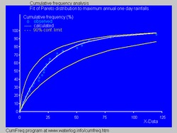
In hydrology the distribution of Pareto applies to extreme events such as the annual maximum rainfall of one day and the discharges of the rivers. and also to describe times of drought. The blue image illustrates an example of adjustment of the distribution of Pareto to the annual maximum precipitations of a classified day also showing the confidence band of 90% based on the binomial distribution. The precipitation data is represented by trace position as part of the analysis of the accumulated frequency.
In the reliability of the distribution of electrical services (80 per cent of the minutes of interrupted customers are produced in approximately 20 per cent of the days of a given year).

Software

Software and a computer program can be used to fit a probability distribution, including a Pareto distribution, to a series of data:

Easy fit Archived on 23 February 2018 in Wayback Machine., "data analysis & simulation"
ModelRisk, "risk modelling software"
Ricci distributions, fitting distrubutions with R, Vito Ricci, 2005
Risksolver, automatically fit distributions and parameters to samples
StatSoft distribution fitting Archived on August 30, 2012 at Wayback Machine.
CumFreq, at no cost, includes confidence intervals based on binomial distribution

Contenido relacionado

Más resultados...