Cauchy distribution

The Cauchy-Lorentz distribution, named after Augustin Cauchy and Hendrik Lorentz, is a continuous probability distribution. It is known as the Cauchy distribution and in physics it is known as the Lorentz distribution, the Lorentzian function or the distribution of Breit-Wigner. Its importance in physics is given by being the solution of the differential equation that describes the forced resonance. In spectroscopy it describes the shape of spectral lines that are broadened by various mechanisms, in particular the collisional broadening mechanism.

Characterization

Density function

In statistics the Cauchy distribution (sometimes also Lorentz distribution) is a continuous probability distribution whose density function is

f(x;x0,γ γ )=1π π γ γ [chuckles]1+(x− − x0γ γ )2]=1π π [chuckles]γ γ (x− − x0)2+γ γ 2]{displaystyle {begin{aligned}f(x;x_{0},gamma) fake={frac {1}{pi gamma left[1+left({frac {x-x}{0}}}}{gamma }{2}{2}{2}{2}{ right}{x1⁄2}{x1⁄2}{x1⁄2}{x1⁄2}}}{x1⁄2}{x1⁄2}{b0}{b1⁄2}{x1⁄2}{b0}{b0}{b0}{b0}{b0}{b0}{b0}{b0}{b0}}}{f)}}}{b0}{b0}{b0}{b0}{b0}{b0}{b0}{b0}}{b)}}{

where x₀ is the shift parameter that specifies the location of the peak of the distribution, and γ is the scale parameter that specifies the half-width at half-maximum (HWHM).

In the special case where x₀ = 0 and γ = 1 is called the standard Cauchy distribution with the probability density function

f(x;0,1)=1π π (1+x2).{displaystyle f(x;0,1)={frac {1}{pi (1+x^{2}}}}}}}}}.

In general, the Cauchy distribution has neither expected value nor variance.

Sean. U{displaystyle U} and V{displaystyle V} two uniform random variables within -1 and 1 and <math alttext="{displaystyle U^{2}+V^{2}U2+V2.1{displaystyle U^{2}+V^{2}{2}{1}<img alt="{displaystyle U^{2}+V^{2}, then the number U/V{displaystyle U/V} has the Cauchy distribution.

Distribution function

The cumulative distribution function (CDF) is:

F(x;x0,γ γ )=1π π arctan (x− − x0γ γ )+12{displaystyle F(x;x_{0},gamma)={frac {1}{pi }}}arctan left({frac {x-x_{0}}}{gamma }}}{right)+{frac {1}{2}}}}}}

and the inverse cumulative distribution function for the Cauchy distribution is

F− − 1(p;x0,γ γ )=x0+γ γ So... [chuckles]π π (p− − 12)].{displaystyle F^{-1}(p;x_{0},gamma)=x_{0}+gamma ,tan left[pi ,left(p-{tfrac {1}{2}}}{2}}{right)right]. !

Properties

The Cauchy distribution is an example of a distribution that has no expected value, variance, or definite moments. Its mode and median are well defined and are both equal to x₀.

When U and V are two independent, normally distributed random variables with expected value = 0 and variance = 1, then the rate U/V has the standard Cauchy distribution.

If X₁, …, X_n are random variables, independent and identically distributed, each with a Cauchy distribution, then the sample mean (X₁ + … + X_n)/n has the same standard Cauchy distribution (the sample mean, which is unaffected by extreme values, can be used as a measure of the central tendency). To verify that this is true, the characteristic function of the sample mean is calculated:

φ φ X! ! (t)=E(eiX! ! t){displaystyle phi _{overline {X}}(t)=mathrm {E} left(e^{i,{overline {X}},t}right),!}

where X! ! {displaystyle {overline {X}}} It's the average sample. This example serves to demonstrate that the hypothesis of finite variance in the theorem of the central boundary cannot be deposed, as does the hypothesis of finite hope in the law of large numbers. It is also an example of a more widespread version of the central limit theorem that is characteristic of all the alpha-estable asymmetrical distributions of Lévy, of which is the distribution of Cauchy a special case.

The Cauchy distribution is an infinitely divisible distribution function. It is also a strictly stable distribution.

The Cauchy distribution matches the Student's t-distribution with one degree of freedom.

Function Characteristic

Let X be a random variable with a Cauchy distribution. Then the characteristic function of the Cauchy distribution is well defined:

φ φ x(t;x0,γ γ )=E(eiXt)=Exp (ix0t− − γ γ 日本語t日本語).{displaystyle phi _{x}(t;x_{0},gamma)=mathrm {E} (e^{i,X,t})=exp(i,x_{0},t-gamma ,int. !

Application of the accumulated probability distribution of Cauchy to maximum dairy rains.

Application

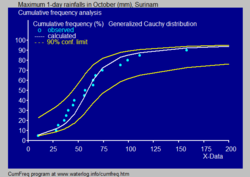
• In hydrology, the distribution of Cauchy is used to analyze random variables as maximum values of precipitation and river discharge, and also to describe times of drought.

The blue image illustrates an example of the adjustment of the Cauchy distribution to the ordered maximum rains daily, also showing the 90% trust strip, based on the binomial distribution. The observations present the position markers, as part of the accumulated frequency analysis.