Antiderivada

ImprimirCitar

Conceito em cálculo

O campo de inclinação de

{displaystyle F(x)={frac {x^{3}}{3}}-{frac {x^{2}}{2}}-x+c}

, mostrando três das infinitamente muitas soluções que podem ser produzidas variando a constante arbitrária

c

No cálculo, uma antiderivada, derivada inversa, função primitiva, integral primitiva ou indefinida integral de uma função $f$ é uma função diferenciável $F$ cuja derivada é igual à função original $f$ . Isso pode ser declarado simbolicamente como $F' = f$ . O processo de resolução de antiderivadas é chamado de antidiferenciação (ou integração indefinida), e sua operação oposta é chamada de diferenciação, que é o processo de encontrar um derivado. Antiderivadas são muitas vezes indicadas por letras romanas maiúsculas, como $F$ e $G$ .

As primitivas estão relacionadas às integrais definidas por meio do segundo teorema fundamental do cálculo: a integral definida de uma função em um intervalo fechado onde a função é Riemann integrável é igual à diferença entre os valores de uma antiderivada avaliada nos pontos finais da intervalo.

Na física, antiderivadas surgem no contexto do movimento retilíneo (por exemplo, ao explicar a relação entre posição, velocidade e aceleração). O equivalente discreto da noção de antiderivada é a antidiferença.

Exemplos

A função ${displaystyle F(x)={tfrac {x^{3}}{3}}}$ é um antiderivado de $f(x)=x^{2}$ , desde o derivado de ${displaystyle {tfrac {x^{3}}{3}}}$ o $x^{2}$ , e como o derivado de uma constante é zero, $x^{2}$ terá um número infinito de antiderivados, como ${displaystyle {tfrac {x^{3}}{3}},{tfrac {x^{3}}{3}}+1,{tfrac {x^{3}}{3}}-2}$ , etc. Assim, todos os antiderivados de $x^{2}$ pode ser obtido alterando o valor de $c$ em ${displaystyle F(x)={tfrac {x^{3}}{3}}+c}$ , onde $c$ é uma constante arbitrária conhecida como a constante de integração. Essencialmente, os gráficos de antiderivados de uma determinada função são traduções verticais uns dos outros, com a localização vertical de cada grafo dependendo do valor $c$ .

Mais geralmente, a função de potência $f(x)=x^{n}$ tem antiderivado ${displaystyle F(x)={tfrac {x^{n+1}}{n+1}}+c}$ se $n \neq -1$ e ${displaystyle F(x)=ln |x|+c}$ se $n = -1$ .

Na física, a integração da aceleração resulta na velocidade mais uma constante. A constante é o termo de velocidade inicial que seria perdido ao tomar a derivada da velocidade, porque a derivada de um termo constante é zero. Esse mesmo padrão se aplica a outras integrações e derivadas de movimento (posição, velocidade, aceleração e assim por diante). Assim, a integração produz as relações de aceleração, velocidade e deslocamento:

{displaystyle {begin{aligned}int a,mathrm {d} t&=v+Cint v,mathrm {d} t&=s+Cend{aligned}}}

Usos e propriedades

Os antiderivados podem ser usados para calcular integrais definitivas, usando o teorema fundamental do cálculo: se $F$ é um antiderivado da função integrable $f$ sobre o intervalo $[a,b]$ Então...

{displaystyle int _{a}^{b}f(x),mathrm {d} x=F(b)-F(a).}

Por causa disso, cada uma das infinitas antiderivadas de uma dada função $f$ pode ser chamada de "integral indefinida" de f e escrito usando o símbolo integral sem limites:

{displaystyle int f(x),mathrm {d} x.}

Se $F$ é um antiderivado de $f$ , e a função $f$ é definido em algum intervalo, então cada outro antiderivativo $G$ de $f$ difere de $F$ por uma constante: existe um número $c$ tal que ${displaystyle G(x)=F(x)+c}$ para todos $x$ . $c$ é chamado de constante de integração. Se o domínio de $F$ é uma união disjunta de dois ou mais intervalos (abertos), então uma constante diferente de integração pode ser escolhida para cada um dos intervalos. Por exemplo

<math alttext="{displaystyle F(x)={begin{cases}-{dfrac {1}{x}}+c_{1}&x0end{cases}}}" display="block" xmlns="http://www.w3.org/1998/Math/MathML">F(x)= = = = = = = = = = = = = = = = = = = = = = = = = = = = = = = = = = = = = = = = = = = = = = = = = = = = = = = = = = = = = = = = = = = = = = = = = = = = = = = = = = = = = = = = = = = = = = = = = = = = = = = = = = = = = = = = = = = = = = = = = = = = = = = = = = = = = = = = = = = = = = = = = = = = = = = = = = = = = = = = = = = = = = = = = = = = = = = = = = = = = = = = = = = = = = = = = = = = = = = = = = = = = = = = = = = = = = = = = = = = = = = = = = = = = = = = = = = = = = = = = = = = = = = = = = = = = = = =(- Sim. - Sim. 1x+c1x<0- Sim. - Sim. 1x+c2x>0F(x)={begin{cases}-{dfrac {1}{x}}+c_{1}&x0end{cases}}}<img alt="{displaystyle F(x)={begin{cases}-{dfrac {1}{x}}+c_{1}&x0end{cases}}}" aria-hidden="true" class="mwe-math-fallback-image-display" src="https://wikimedia.org/api/rest_v1/media/math/render/svg/60dc09aa2f12fedbfbe454d8e86433b2aa341ca0" style="vertical-align: -5.171ex; width:27.584ex; height:11.509ex;"/>

é o antiderivativo mais geral de $f(x)=1/x^{2}$ em seu domínio natural ${displaystyle (-infty0)cup (0,infty).}$

Toda função contínua $f$ tem uma antiderivada e uma antiderivada $F$ é dado pela integral definida de $f$ com limite superior variável:

{displaystyle F(x)=int _{0}^{x}f(t),mathrm {d} t.}

Existem muitas funções cujas primitivas, embora existam, não podem ser expressas em termos de funções elementares (como polinômios, funções exponenciais, logaritmos, funções trigonométricas, funções trigonométricas inversas e suas combinações). Exemplos disso são

a função de erro ${displaystyle int e^{-x^{2}},mathrm {d} x,}$
a função Fresnel ${displaystyle int sin x^{2},mathrm {d} x,}$
a integral do pecado ${displaystyle int {frac {sin x}{x}},mathrm {d} x,}$
a função integral logarítmica ${displaystyle int {frac {1}{ln x}},mathrm {d} x,}$ e
Sonho do sophomore ${displaystyle int x^{x},mathrm {d} x.}$

Para uma discussão mais detalhada, veja também a teoria diferencial de Galois.

Técnicas de integração

Encontrar antiderivadas de funções elementares costuma ser consideravelmente mais difícil do que encontrar suas derivadas (de fato, não há um método predefinido para calcular integrais indefinidas). Para algumas funções elementares, é impossível encontrar uma antiderivada em termos de outras funções elementares. Para saber mais, consulte funções elementares e integral não elementar.

Existem muitas propriedades e técnicas para encontrar antiderivadas. Estes incluem, entre outros:

A linearidade da integração (que quebra integrais complicadas em integrais mais simples)
Integração por substituição, muitas vezes combinada com identidades trigonométricas ou o logaritmo natural
O método de regra da cadeia inversa (um caso especial de integração por substituição)
Integração por partes (para integrar produtos de funções)
Integração da função inversa (uma fórmula que expressa o antiderivado do inverso $f - Sim.$ de uma função invertível e contínua $f$ , em termos do antiderivado de $f$ de $f - Sim.$ ).
O método de frações parciais na integração (que nos permite integrar todas as funções racionais - frações de dois polinômios)
O algoritmo de Risch
Técnicas adicionais para múltiplas integrações (veja, por exemplo, integrais duplas, coordenadas polares, o teorema de Jacobiano e os Stokes)
Integração numérica (uma técnica para aproximar uma integral definida quando nenhuma antiderivativa elementar existe, como no caso de $exp(- x 2)$ )
Manipulação algébrica do integrando (para que outras técnicas de integração, como integração por substituição, possam ser utilizadas)
Fórmula de Cauchy para integração repetida (para calcular a $n$ -tempos antiderivados de uma função) ${displaystyle int _{x_{0}}^{x}int _{x_{0}}^{x_{1}}cdots int _{x_{0}}^{x_{n-1}}f(x_{n}),mathrm {d} x_{n}cdots ,mathrm {d} x_{2},mathrm {d} x_{1}=int _{x_{0}}^{x}f(t){frac {(x-t)^{n-1}}{(n-1)!}},mathrm {d} t.}$

Sistemas de álgebra computacional podem ser usados para automatizar parte ou todo o trabalho envolvido nas técnicas simbólicas acima, o que é particularmente útil quando as manipulações algébricas envolvidas são muito complexas ou demoradas. As integrais que já foram derivadas podem ser consultadas em uma tabela de integrais.

De funções não contínuas

Funções não contínuas podem ter antiderivadas. Embora ainda existam questões em aberto nesta área, sabe-se que:

Algumas funções patológicas altamente com grandes conjuntos de descontinuidades podem, no entanto, ter antiderivativos.
Em alguns casos, os antiderivados de tais funções patológicas podem ser encontrados pela integração de Riemann, enquanto em outros casos essas funções não são integrais de Riemann.

Assumindo que os domínios das funções são intervalos abertos:

Uma condição necessária, mas não suficiente para uma função $f$ ter um antiderivado é que $f$ tem a propriedade de valor intermediário. Isso é, se $Não. um, b)]$ é uma subinterval do domínio de $f$ e $Sim.$ é um número real entre $f (um)$ e $f (b))$ , então existe uma $c$ entre $um$ e $b)$ tal que $f (c) = Sim.$ . Isto é uma consequência do teorema de Darboux.
O conjunto de descontinuidades $f$ deve ser um conjunto minucioso. Este conjunto também deve ser um conjunto F-sigma (uma vez que o conjunto de descontinuidades de qualquer função deve ser deste tipo). Além disso, para qualquer conjunto de F-sigma meagre, pode-se construir alguma função $f$ ter um antiderivativo, que tem o conjunto dado como seu conjunto de descontinuidades.
Se $f$ tem um antiderivativo, é limitado em subintervalos finitos fechados do domínio e tem um conjunto de descontinuidades da medida Lebesgue 0, então um antiderivativo pode ser encontrado pela integração no sentido de Lebesgue. De fato, usando integrais mais poderosas como a integral Henstock-Kurzweil, cada função para a qual existe uma antiderivativa é integravel, e sua integral geral coincide com sua antiderivativa.
Se $f$ tem um antiderivativo $F$ em um intervalo fechado $[a,b]$ , então para qualquer escolha de partição $<math alttext="{displaystyle a=x_{0}<x_{1}<x_{2}<dots um= = = = = = = = = = = = = = = = = = = = = = = = = = = = = = = = = = = = = = = = = = = = = = = = = = = = = = = = = = = = = = = = = = = = = = = = = = = = = = = = = = = = = = = = = = = = = = = = = = = = = = = = = = = = = = = = = = = = = = = = = = = = = = = = = = = = = = = = = = = = = = = = = = = = = = = = = = = = = = = = = = = = = = = = = = = = = = = = = = = = = = = = = = = = = = = = = = = = = = = = = = = = = = = = = = = = = = = = = = = = = = = = = = = = = = = = = = = = = = = = = = = = = = = = = = = = = = = =x0<x1<x2<⋯ ⋯ <xn= = = = = = = = = = = = = = = = = = = = = = = = = = = = = = = = = = = = = = = = = = = = = = = = = = = = = = = = = = = = = = = = = = = = = = = = = = = = = = = = = = = = = = = = = = = = = = = = = = = = = = = = = = = = = = = = = = = = = = = = = = = = = = = = = = = = = = = = = = = = = = = = = = = = = = = = = = = = = = = = = = = = = = = = = = = = = = = = = = = = = = = = = = = = = = = = = = = = = = = = = = = = = = = = = = = = = = = = = = = = = = = = = = = = = = = = = = = = = = = = = = = = = = = = = = = = = = = =b),{displaystyle a=x_{0}<x_{1}<x_{2}<dots <x_{n}=b,}<img alt="{displaystyle a=x_{0}<x_{1}<x_{2}<dots$ se alguém escolher pontos de amostra $x_{i}^{*}in [x_{i-1},x_{i}]$ como especificado pelo teorema de valor médio, então os telescópios de soma Riemann correspondentes ao valor ${displaystyle F(b)-F(a)}$ . ${displaystyle {begin{aligned}sum _{i=1}^{n}f(x_{i}^{*})(x_{i}-x_{i-1})&=sum _{i=1}^{n}[F(x_{i})-F(x_{i-1})]&=F(x_{n})-F(x_{0})=F(b)-F(a)end{aligned}}}$ Contudo, se $f$ é unbounded, ou se $f$ é limitado, mas o conjunto de descontinuidades de $f$ tem medida Lebesgue positiva, uma escolha diferente de pontos de amostra $x_{i}^{*}$ pode dar um valor significativamente diferente para a soma de Riemann, não importa quão fina a partição. Veja Exemplo 4 abaixo.

Alguns exemplos

The function
${displaystyle f(x)=2xsin left({frac {1}{x}}right)-cos left({frac {1}{x}}right)}$ with $f(0)=0$ is not continuous at $x=0$ but has the antiderivative ${displaystyle F(x)=x^{2}sin left({frac {1}{x}}right)}$
with $F(0)=0$ . Since $f$ is bounded on closed finite intervals and is only discontinuous at 0, the antiderivative $F$ may be obtained by integration: $F(x)=int _{0}^{x}f(t),mathrm {d} t$ .
The function ${displaystyle f(x)=2xsin left({frac {1}{x^{2}}}right)-{frac {2}{x}}cos left({frac {1}{x^{2}}}right)}$ with $f(0)=0$ is not continuous at $x=0$ but has the antiderivative ${displaystyle F(x)=x^{2}sin left({frac {1}{x^{2}}}right)}$ with $F(0)=0$ . Unlike Example 1, $f (x)$ is unbounded in any interval containing 0, so the Riemann integral is undefined.
If $f (x)$ is the function in Example 1 and $F$ is its antiderivative, and ${x_{n}}_{ngeq 1}$ is a dense countable subset of the open interval ${displaystyle (-1,1),}$ then the function ${displaystyle g(x)=sum _{n=1}^{infty }{frac {f(x-x_{n})}{2^{n}}}}$ has an antiderivative ${displaystyle G(x)=sum _{n=1}^{infty }{frac {F(x-x_{n})}{2^{n}}}.}$ The set of discontinuities of $g$ is precisely the set ${displaystyle {x_{n}}_{ngeq 1}}$ . Since $g$ is bounded on closed finite intervals and the set of discontinuities has measure 0, the antiderivative $G$ may be found by integration.
Let ${x_{n}}_{ngeq 1}$ be a dense countable subset of the open interval ${displaystyle (-1,1).}$ Consider the everywhere continuous strictly increasing function ${displaystyle F(x)=sum _{n=1}^{infty }{frac {1}{2^{n}}}(x-x_{n})^{1/3}.}$ It can be shown that ${displaystyle F'(x)=sum _{n=1}^{infty }{frac {1}{3cdot 2^{n}}}(x-x_{n})^{-2/3}}$

Figure 1.

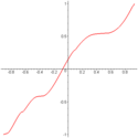Figure 2.

for all values $x$ where the series converges, and that the graph of $F (x)$ has vertical tangent lines at all other values of $x$ . In particular the graph has vertical tangent lines at all points in the set ${displaystyle {x_{n}}_{ngeq 1}}$ .
Moreover ${displaystyle F(x)geq 0}$ for all $x$ where the derivative is defined. It follows that the inverse function ${displaystyle G=F^{-1}}$ is differentiable everywhere and that
${displaystyle g(x)=G'(x)=0}$
for all $x$ in the set ${F(x_{n})}_{ngeq 1}$ which is dense in the interval ${displaystyle [F(-1),F(1)].}$ Thus $g$ has an antiderivative $G$ . On the other hand, it can not be true that
${displaystyle int _{F(-1)}^{F(1)}g(x),mathrm {d} x=GF(1)-GF(-1)=2,}$
since for any partition of ${displaystyle [F(-1),F(1)]}$ , one can choose sample points for the Riemann sum from the set ${F(x_{n})}_{ngeq 1}$ , giving a value of 0 for the sum. It follows that $g$ has a set of discontinuities of positive Lebesgue measure. Figure 1 on the right shows an approximation to the graph of $g (x)$ where ${x_{n}=cos(n)}_{ngeq 1}$ and the series is truncated to 8 terms. Figure 2 shows the graph of an approximation to the antiderivative $G (x)$ , also truncated to 8 terms. On the other hand if the Riemann integral is replaced by the Lebesgue integral, then Fatou's lemma or the dominated convergence theorem shows that $g$ does satisfy the fundamental theorem of calculus in that context.
In Examples 3 and 4, the sets of discontinuities of the functions $g$ are dense only in a finite open interval ${displaystyle (a,b).}$ However, these examples can be easily modified so as to have sets of discontinuities which are dense on the entire real line $(-inftyinfty)$ . Let ${displaystyle lambda (x)={frac {a+b}{2}}+{frac {b-a}{pi }}tan ^{-1}x.}$ Then ${displaystyle g(lambda (x))lambda '(x)}$ has a dense set of discontinuities on $(-inftyinfty)$ and has antiderivative $Gcdot lambda.$
Using a similar method as in Example 5, one can modify $g$ in Example 4 so as to vanish at all rational numbers. If one uses a naive version of the Riemann integral defined as the limit of left-hand or right-hand Riemann sums over regular partitions, one will obtain that the integral of such a function $g$ over an interval $[a,b]$ is 0 whenever $a$ and $b$ are both rational, instead of ${displaystyle G(b)-G(a)}$ . Thus the fundamental theorem of calculus will fail spectacularly.
A function which has an antiderivative may still fail to be Riemann integrable. The derivative of Volterra's function is an example.

Fórmulas básicas

Se ${displaystyle {mathrm {d} over mathrm {d} x}f(x)=g(x)}$ , então ${displaystyle int g(x)mathrm {d} x=f(x)+C}$ .
${displaystyle int 1 mathrm {d} x=x+C}$
${displaystyle int a mathrm {d} x=ax+C}$
${displaystyle int x^{n}mathrm {d} x={frac {x^{n+1}}{n+1}}+C; nneq -1}$
${displaystyle int sin {x} mathrm {d} x=-cos {x}+C}$
${displaystyle int cos {x} mathrm {d} x=sin {x}+C}$
${displaystyle int sec ^{2}{x} mathrm {d} x=tan {x}+C}$
${displaystyle int csc ^{2}{x} mathrm {d} x=-cot {x}+C}$
${displaystyle int sec {x}tan {x} mathrm {d} x=sec {x}+C}$
${displaystyle int csc {x}cot {x} mathrm {d} x=-csc {x}+C}$
${displaystyle int {frac {1}{x}} mathrm {d} x=ln |x|+C}$
${displaystyle int e^{x}mathrm {d} x=e^{x}+C}$
$0, aneq 1}" xmlns="http://www.w3.org/1998/Math/MathML">∫ ∫ umxDx= = = = = = = = = = = = = = = = = = = = = = = = = = = = = = = = = = = = = = = = = = = = = = = = = = = = = = = = = = = = = = = = = = = = = = = = = = = = = = = = = = = = = = = = = = = = = = = = = = = = = = = = = = = = = = = = = = = = = = = = = = = = = = = = = = = = = = = = = = = = = = = = = = = = = = = = = = = = = = = = = = = = = = = = = = = = = = = = = = = = = = = = = = = = = = = = = = = = = = = = = = = = = = = = = = = = = = = = = = = = = = = = = = = = = = = = = = = = = = = = = = = = = = = = = = = = = = = =umxI⁡ ⁡ um+C;um>0,um≠ ≠ 1{displaystyle int a^{x}mathrm {d} x={frac {a^{x}}{ln a}}+C; a>0, aneq 1}0, aneq 1}" aria-hidden="true" class="mwe-math-fallback-image-inline" src="https://wikimedia.org/api/rest_v1/media/math/render/svg/80c0091fa01431d9a4bf28789dcb8898866d0158" style="vertical-align: -2.338ex; width:33.914ex; height:5.676ex;"/>$